A taxonomy of open source software

TL;DR: We created a data-driven taxonomy of software projects by performing NLP on READMEs and metadata. Our results on 1M GitHub repos show that our automated labelling algorithms can reduce the number of unique topic labels by a factor of 400x and decrease the number of unlabelled projects by 7x. We released a fun visual representation of our taxonomy that devs can use to explore the space of OSS and to provide a portrait of their own experience.

Open source software (OSS) enables or assists nearly every aspect of human activity, including software for computer operating systems, fundamental physics research, AI, and much more besides. It is hard to keep track of the many projects one encounters. The many layers of abstraction and the wide variety of domains make it difficult to comprehend both unfamiliar projects and the ecosystem as a whole. This problem is amplified by the vast numbers of people who contribute to OSS development, while also paradoxically making their contributions less visible. For us at Quine this is a fundamental problem, especially as we design algorithms to quantify the reputation and experience of software developers.

In this post we discuss our efforts to systematically categorize open-source projects via machine learning (ML). To do this, we’ve constructed a taxonomy of OSS from GitHub data. We automatically generate labels for software projects based on their README files and metadata via natural language processing (NLP). The taxonomy is already a central component of our product, so in this post we dive into the technical details behind it and discuss how it unlocks some new visualizations of the open source ecosystem, and novel search interfaces for repos and developers. If you want to skip the details and go straight to the fun, you can play around with our taxonomy by clicking on this link 👈.

Introduction

Encountering a new project in open source can be a daunting experience. A key problem is contextualization. For example: what problem is this project solving? What area does it belong to? Do these keywords help my understanding, or are they false friends? Is it an isolated repository, or are there thousands like it? Is there a popular alternative with better documentation and maintenance? The manual solution (searching, Q&A sites) to this problem doesn’t scale well when considering the millions of projects in the OSS space. A practical option for many is to find an appropriate high-level label, such as devops or security, and throw the project onto a mental heap of other loosely associated projects. This ‘problem’ of new projects extends even to specialists: keeping on top of progress in a domain can be hard work, a problem that is dramatically worsened when returning after a hiatus.

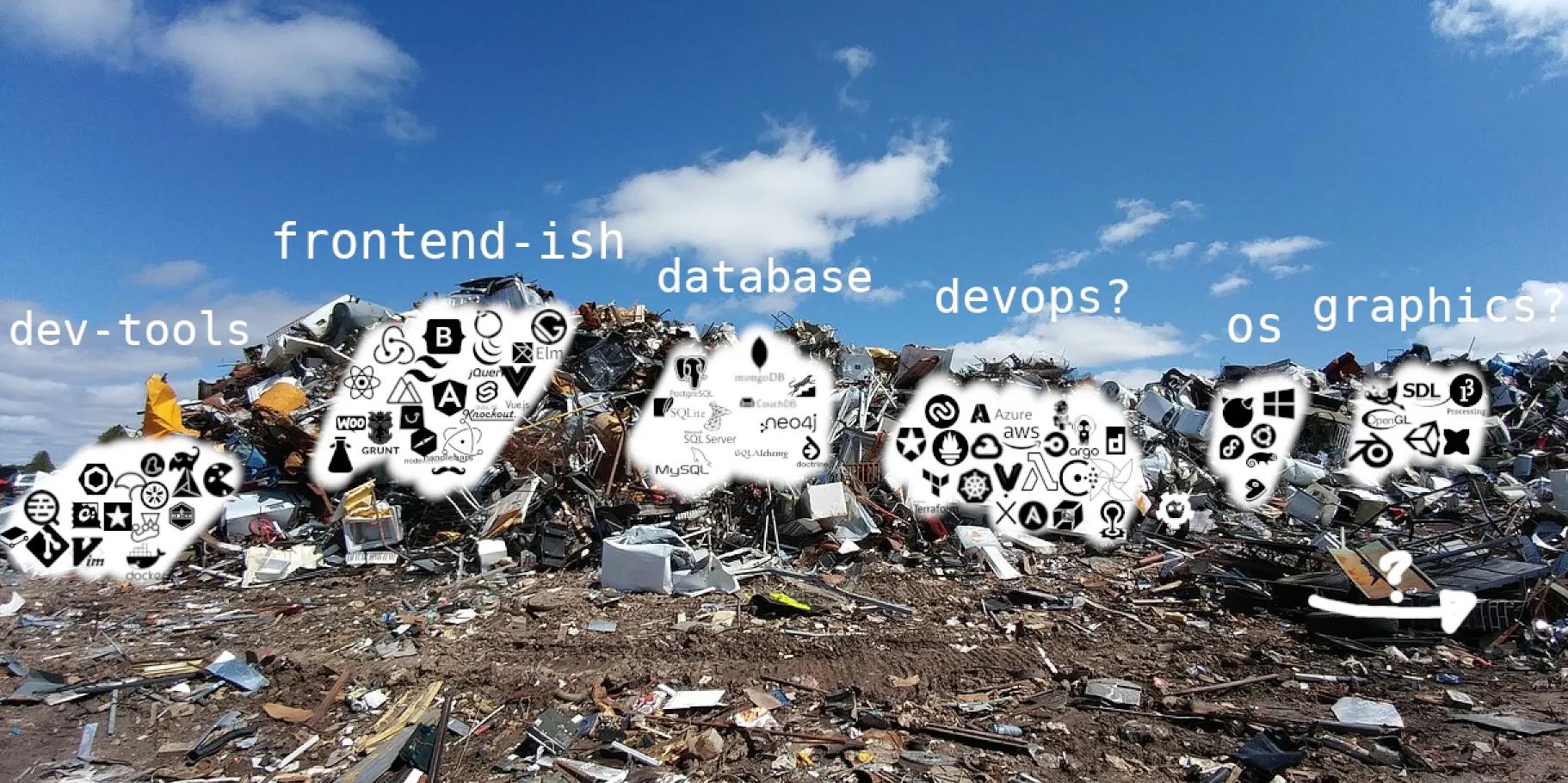
Photography credit: Pixabay/vkingxl

A notable deficiency of OSS in this context is a reliable form of systematic categorization. There are existing tools to help us in this space, but none without significant problems. For example one can use a taxonomy within a package registry (e.g. PyPI) or repository hosting platform (e.g. SourceForge), or a folksonomy (i.e. free-text tagging, as found on e.g. npm or GitHub). But these existing tools suffer from two substantial shortcomings. Firstly and most importantly, they assume people want to tag their work and are doing it in a helpful manner. As it turns out, the majority of projects are not labelled (see below), and even when they are, it is done inconsistently, and suffers from various reporting biases. Secondly, to the best of our knowledge, existing taxonomies are not comprehensive — either by design or because they fall out-of-date; folksonomies suffer from an equal and opposite problem: lack of standardization, proliferation of labels, and ambiguous or overloaded terms.

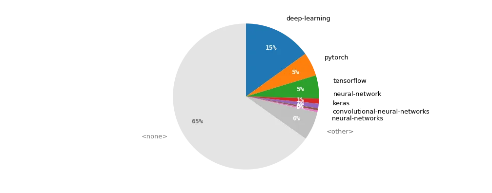
The labels provided by GitHub owners of projects our taxonomy deems as “deep-learning”. Where multiple relevant labels are present, we choose the most popular; “<other>” encompasses more than 450 relevant tags.

Consider the case of ‘deep learning’: a large, and enormously important field for AI and related tools. One will not find projects tagged with this label in either PyPI or SourceForge; it doesn’t exist, at least at the time of writing. Within the folksonomies such as GitHub, one can search, but one needs to consider the union of many keywords, such as deep-learning, automatic-differentiation, neural-network, neural-networks, deep-neural-network, and possibly tensorflow, pytorch, jax, mxnet, etc. And due to the lack of tagging, or standardization thereof, the overwhelming majority (in this case 65–70%) of relevant projects will still not be present.

Now consider the outcome if such labels were de-duplicated appropriately, and the majority of relevant projects were automatically tagged? We would no longer need blogs describing the “top 10 tools for X” (which provoke questions such as “how fresh is this?” and “how biased is this?”) and would allow good answers to intersection queries such as “Deep Learning for Music”, or “Fluid Dynamics for Unity”. Such an enterprise is our present goal. The only real options for such queries at the moment are search engines, but one rarely achieves a comprehensive overview, nor an easy way to filter based on popularity or maintenance.

There are other benefits of organizing and labelling OSS too. For instance, developers new to a field may benefit from a mental map and better visibility of important projects. It can also help to solve the “discoverability” problem for creators — if a project is not already popular, and not from a big name developer, it can be an uphill battle to gain the interest of the community.

In the next section we’ll discuss the core tools we’ve developed for these problems; specifically a clean, up-to-date taxonomy which can label projects automatically via use of ML.

Our taxonomy

To summarize, we are looking to provide a tool that promotes accessibility of OSS: to find relevant resources and projects, to aid those wanting to contribute, to help developers understand the contributions of others, and to find other devs with whom to collaborate. This section describes some high-level properties of the taxonomy before we discuss some applications.

Properties:

At a high level our taxonomy achieves:

a comprehensive coverage of all significant areas of OSS (we consider all labels on GitHub with more than 5 tagged repos; c. 40,000 labels)
a reduction in the number of unique labels by a factor of ~400 (from over 240,000 to 600)
unambiguous and distinct topic names which can be rolled up into higher level categories
automatic inference of topic labels for any open source project¹
a data-driven framework to add to or modify branches²

Due to the requirement of topic inference, the taxonomy construction itself is very challenging. It is not sufficient to simply choose sensible topic names (such as shader, ray-tracing and rendering) and locate them within a higher level area (e.g. 3d graphics). Instead, each topic itself comprises child concepts and named entities that (insofar as possible) are mutually exclusive (in order to permit fine-grained inference) and — in combination — must achieve our goal of comprehensively covering the space. Some practical details of our method are provided later.

These properties offer a dramatic improvement in utility beyond that found in existing taxonomies and folksonomies. Unlike existing taxonomies, it reflects the dominant interests in OSS in the present day, and provides a comprehensive labelling of the entire space.³ And unlike folksonomies, we can solve the “freshness” problem without resorting to tens of thousands of non-standardized and esoteric labels. Through use of data science, our approach can re-group and de-duplicate labels, and (semi-)automatic analysis of up-to-date data can provide a solution to the “freshness” problem. Importantly, we label projects automatically, which permits retrieval of the majority of related projects even when there are no tags. To the best of our knowledge, our taxonomy is the first with these properties for open source software.

The taxonomy

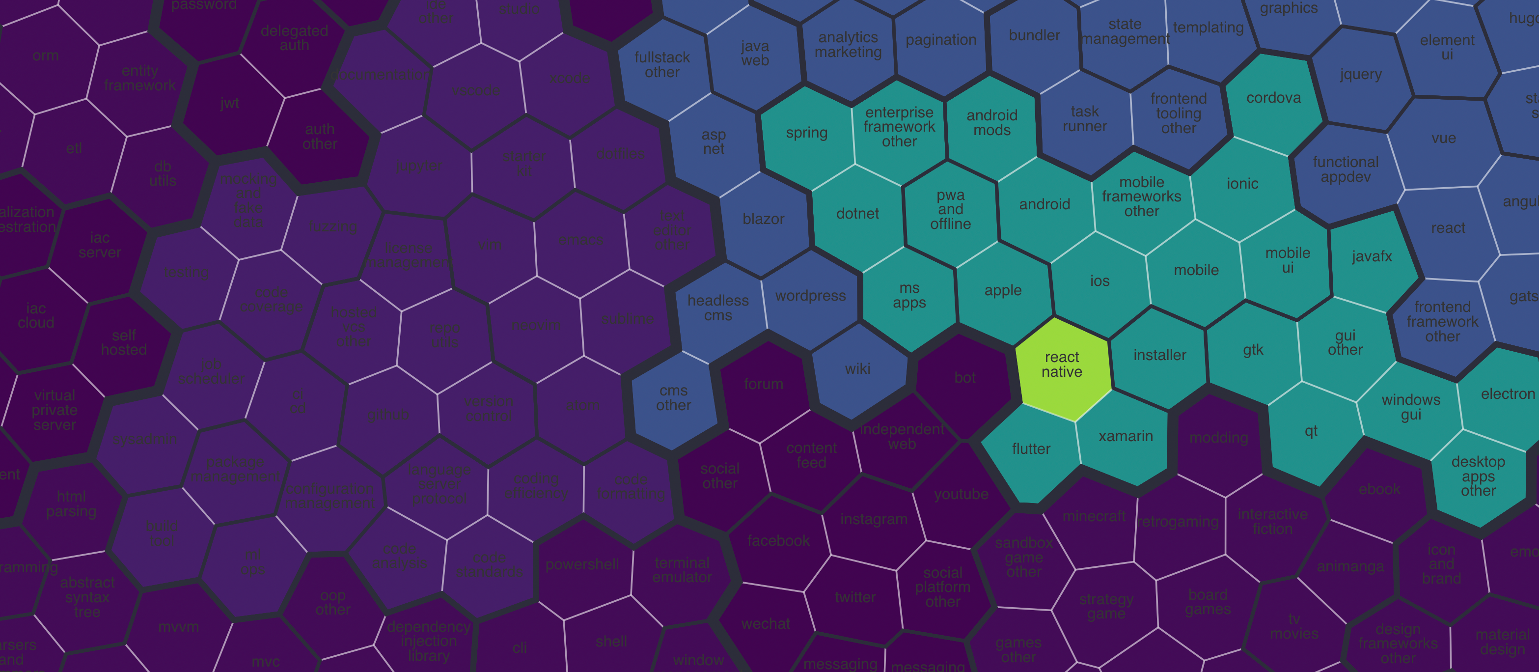
The figure below shows a high-level tree view of the taxonomy, which has approximately 600 topics. The topic areas are a result of analyzing and clustering GitHub topic labels, and are typically either a specialism (e.g. osdev), the ecosystem of a single technology (e.g. react), or an application area (e.g. sport). Certain areas are excluded from the scope — for example information about programming language or runtime which is freely available elsewhere.⁴ Choosing the number of topics is a trade-off between precise topic specification (more topics) and user experience (less topics). Similar topics are recursively grouped via semantic embeddings and positioned within a hierarchical taxonomy; we also applied some fine tuning.

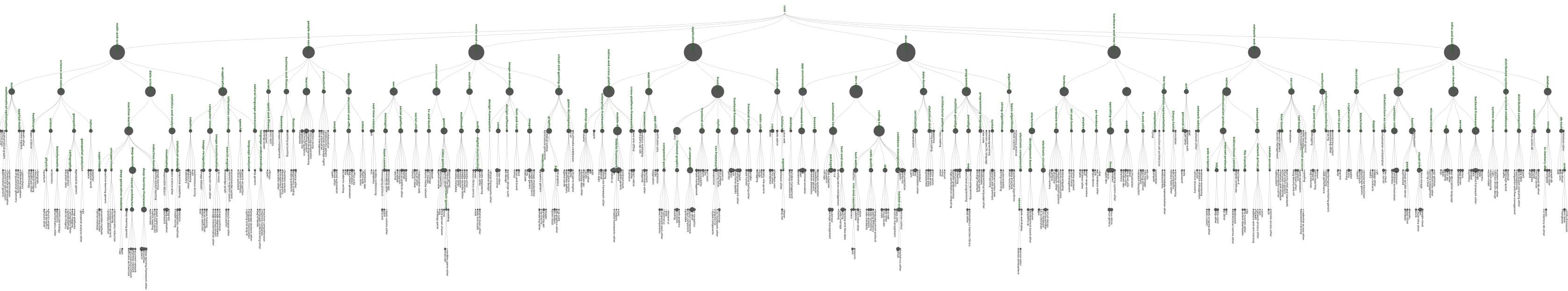
Our taxonomy; take a closer look using this visualization.

For labelling projects we used an ensemble of bespoke models. The scarcity and inaccuracy of existing labels make this a challenging problem: inferring each topic is a fine-grained one-class classification problem with a high level of both label noise and reporting bias. For this reason we tried to avoid placing too much weight on the labels given by users, bootstrapping our inference from a variety of techniques within the unsupervised and semi-supervised learning field. In the interest of time, we will save further details for a possible future post on this subject.

Within our subset of interest⁵, 73% of projects are unlabelled on GitHub, which compares to only 10% of projects using our automated labelling approach. Many of the remaining unlabelled projects are due to poorly written README files, some others are utilities that fall outside the current scope of the taxonomy. Our topic labels are also more concise than those on GitHub, perhaps due to the fact that authors sometimes account for the multiplicity of keywords and pairwise combinations that users may search for.

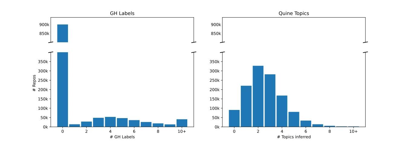
Coverage of GitHub topic labels vs our inferred topics: number of labels per repository.

Examples of use

There are a wide variety of uses of this taxonomy: we provide four here, but we’re exploring a few more within Quine.

Information retrieval for projects

An immediate application of this taxonomy is for use in thematic browsing of open source projects. While some organizations are currently looking at recommendation for OSS (including ourselves), we believe targeted browsing can be more useful. To demonstrate what our index allows, let’s look at the example of molecular-biology. It’s hard to find a reliable list of tools in this space at present, and if one were to search relevant tags on GitHub, one would currently find perhaps only 35 / 100 of our top listed tools. For our top 20 ranked projects, shown below, any project with a “❌” in the “labelled” column would not be retrieved (at the time of writing) when browsing projects under GitHub’s folksonomy for relevant tags. For example, AlphaFold has no labels at all on GitHub (at the time of writing) and so could not be found under a relevant topic search there.

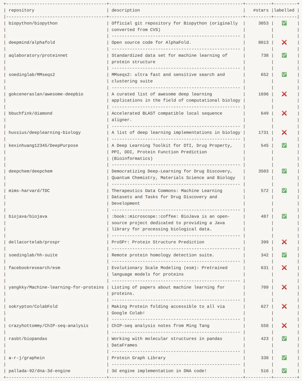
Molecular-biology: top 20 projects according to our automated taxonomy inference

More flexible options for browsing in this way are available at https://quine.sh/d/find-tools, where we semantically index 150,000 of the most popular GitHub projects. We intend to grow the index significantly over the coming months.

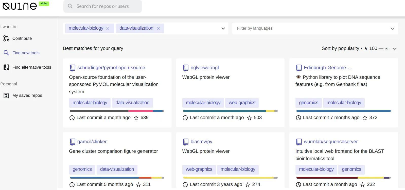
Browsing GitHub projects at https://quine.sh/d/find-tools

Browsing / finding developers

Another information retrieval application is in browsing top developers for a topic. This might be useful for finding developers to follow, or to work with. This is not facilitated by GitHub, and would not be advisable anyway, since most work that a developer does is not tagged, or not tagged in a standardized way. Using the repos scored against our taxonomy, we can create a score for a (developer, topic) tuple, for example, as a function of the number of contributions to relevant projects, the topic score we assign, and the popularity of that project (via GitHub stars). See examples below for testing and circuit-design. These results consider contributions to any repository with ≥ 10 stars; in the table ‘#commits’ is the total number of commits made; ‘#repos’ is the number of distinct projects.

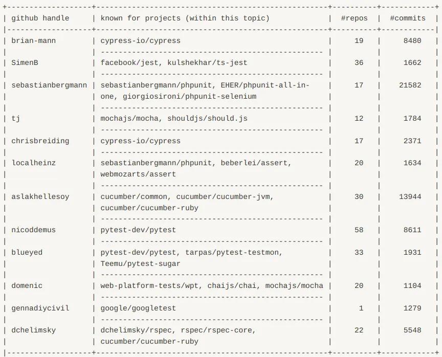
Testing: top 12 developers according to our automated taxonomy inference

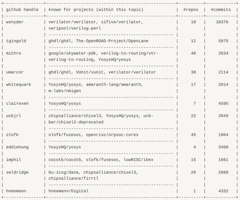
Circuit-design: top 12 developers according to our automated taxonomy inference.

Visual profiles: developers

Developers can be described by their skills (as demonstrated through contributions) but also their interests and learning aspirations. Our taxonomy allows us to combine and locate these aspects on a standardized 2D topic map, creating a visual summary. Examples are given below for some well known OSS developers; here we focus just on open source contributions.

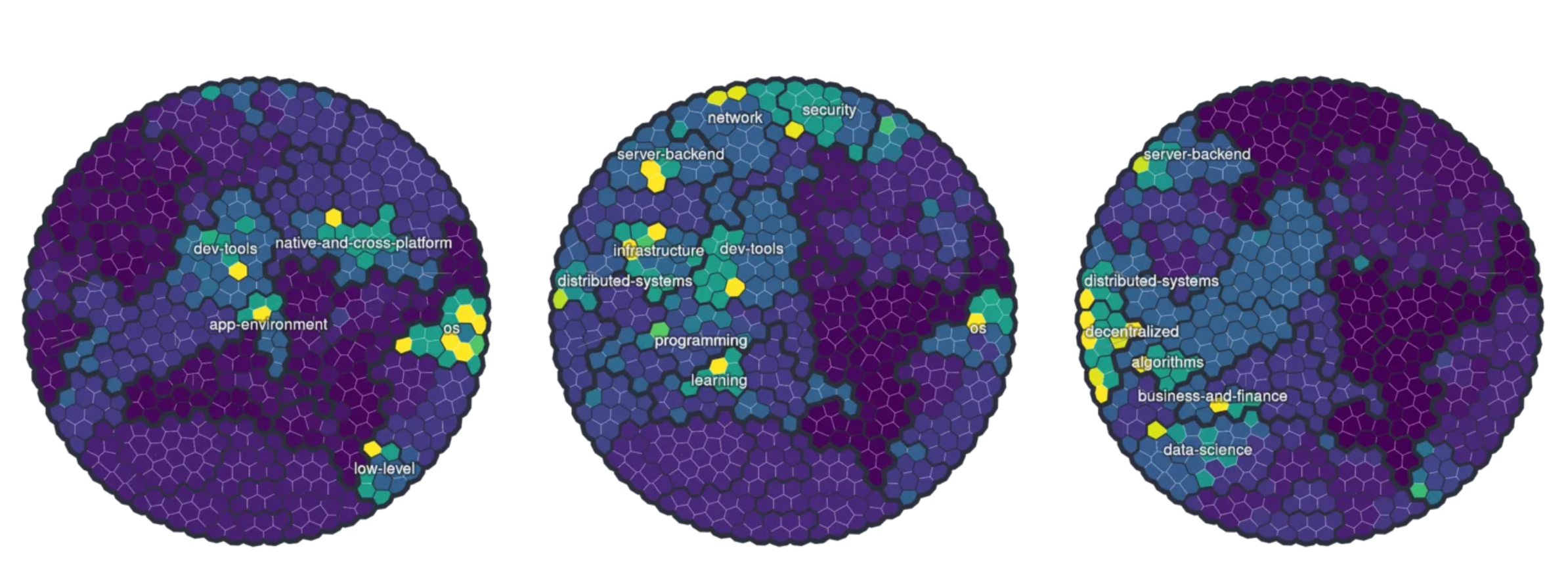
Developer profiles: Linus Torvalds (Linux); Kelsey Hightower (Kubernetes); Jeffrey Wilcke (Ethereum)

Visual profiles: programming languages

Different domains tend to favour different programming languages. These are largely known within the community (such as frontend — Javascript; embedded — C/C++; iOS — Swift; data science — Python), but we can use our topic map to provide a more comprehensive visual overview.

In the following plots, we show the proportion of each language associated with the various topic areas, normalized by the size of each topic (log scale). We pass the result through a sigmoid function since the domain is otherwise the entire real line. The result is heavily related to pointwise mutual information between the topic of a repo and its language.

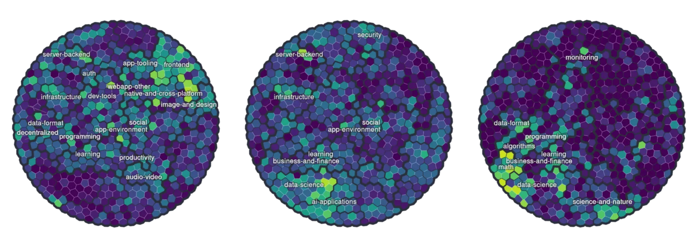
Language profiles: JavaScript; Python; Julia

That’s about it for the pretty pictures. In the final couple of sections of this blog, we’ll try to shed a bit more light on our methods of creating this taxonomy.

Methods

This section elaborates on how we derived the above assets, and is more technical in nature than the discussion so far. At a high-level this consisted of a data-informed, machine-learning-assisted manual effort in annotating and categorizing the space. Creating the taxonomy is a sensitive activity, and can be viewed as a kind of ‘meta-labelling’: the presence of a label within a topic can result in the automated tagging of many thousands of additional OSS projects downstream. Here we provide more details about that journey: our data, approach, and reasoning for the task of constructing the taxonomy; as well as an overview of how we created the topic map.

The first step in constructing the taxonomy is obtaining data. For our present version, we focus on analyzing projects hosted by GitHub, and specifically projects with ≥ 10 stars with English README files (c. 1m repositories).⁶ In particular we focused on the README files, descriptions and user-tagged topics of these projects, obtained via use of GitHub’s API. The decision to focus on GitHub is due to its status as the de facto leader in OSS hosting, and the assumption that it contains a representative sample of OSS. In future, we would like to expand beyond this; but our work on GitHub should transfer directly to projects hosted on other platforms such as GitLab and Bitbucket.

Due to the importance and sensitivity of the task, human verification and fine-tuning is likely essential, whatever the approach. Our intention was therefore to find the simplest method that worked well, rather than spend time developing a complex end-to-end model for the task. Existing work in automated taxonomy construction (see e.g. Wang et al., 2017) usually performs a two-stage process: extract “is-a” relations from natural text, and then construct a hierarchical graph, often by a form of clustering. In our case, we have something similar to relations already: existing labels within the GitHub folksonomy. We also suggest that extracting “is-a”-type relations could be too restrictive for our purposes. For instance, a project tagged with microphone is software which most likely performs some kind of audio engineering, but a microphone itself “is-a” piece of audio hardware.

Our approach is thus to use the existing topic labels from user tags and cluster them into standardized groups. Once done, we can then manually inspect and tune clusters, and thereafter construct a hierarchical graph from them. The candidate set of labels that we consider are GitHub topics with ⪆ 5 uses in our dataset (c. 40,000 unique labels). The frequency of label usage drops off rapidly (see the figure below) and we assume that all “important” concepts are covered within this set. In considering this large candidate set, we remove the bias of keyword popularity: a topic area can be constructed from a single very popular label, or many less-popular labels.

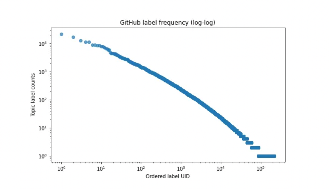
GitHub labels have a long tail, approximately following a Zipf law

Automatic label organization

Our first question was whether the number of topics can be substantially reduced by standard lexicographical analysis. E.g. tokenization, spellchecking etc. We chose to answer this question with a ‘no’. For instance wsus (Windows Server Update Services) is very close to asus in edit distance, but very different in meaning. There are many compound tokens (e.g. machine-learning, haskell-learning) that may be broken down to consistuent parts, but we were unable to reliably tell when this was permissible. As another example, stemming proved problematic (e.g. for Snowball stemming, we have visualize → visual, or worse, ios→ io).

The next simplest approach we considered was the label co-occurrences within each project: it is reasonable to assume that labels which are highly related occur together more often than expected. To this end, a natural metric to consider is pointwise mutual information (PMI), defined between two topics t_a and t_b as:

which is the log of the ratio between the actual co-occurrence of two topics and the expected co-occurrence if they were independent. This can be interpreted as quantifying similarity: we have PMI ≈ 0 when there is no similarity between labels and a larger PMI when the similarity is strong. The required pairwise and marginal distributions are easy to derive from the above dataset, but due to the quadratic number of distributions required, we used GPUs to parallelize the operation.

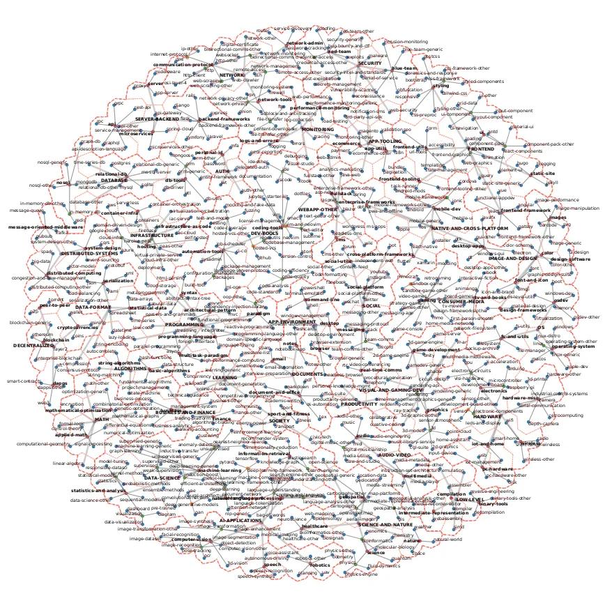
Consider now the graph obtained from the label set, with weighted edges (propotional to PMI) added when PMI > 0. We also chose to give the nodes weights proportional to the logarithm of their label frequency. Finding clusters of similar topics can now be framed as a form of community detection, which we eventually performed via matrix decomposition and weighted k-means with K=500 clusters.⁷

A small subset of the weighted graph of candidate labels visualized via d3-force: edge weight differences can be inferred from their width.

At this stage, we encountered a problem with the use of label co-occurrences: clusters which best represent the data do not necessarily best represent the semantics. As an example, labels similar to interactive-fiction are located near or with terminal. This is a real phenomenon of the data, not a problem with the algorithm, but we do not wish our taxonomy to locate these concepts together. This kind of problem is common, e.g. sports with data-science, gan with computer-vision, or nas (network attached storage) with home-media.

While these problematic correlations exist for the labels, we don’t expect to find these problems to the same extent in natural text. Hence we augmented the graph’s edge weights with semantic similarities of labels based on word2vec embeddings (Mikolov et al., 2013), trained on the README files. This modification demonstrated substantial improvements in cluster coherence. We then constructed the taxonomy based on a hierarchical clustering of the (weighted-)mean embeddings of each topic cluster. We found the results adequate for the purposes of manual review. Some direct results of this are shown in the images below.

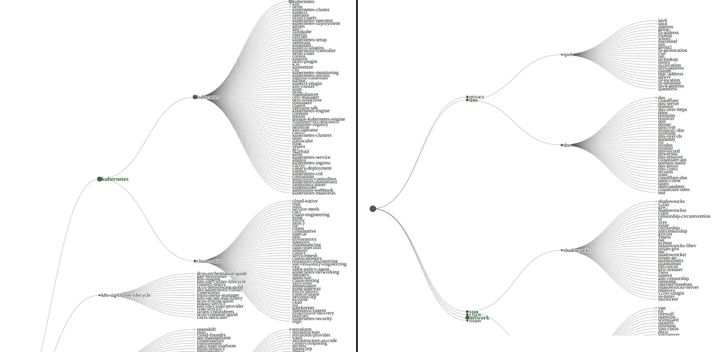
Examples of automatic topic extraction and organization. (Interior nodes are named automatically as the medoid labels of its leaves, and may not be optimal.) LHS - suboptimal: Clusters contain lots of related concepts, but are not entirely coherent. RHS — reasonable: largely coherent and well-positioned clusters.

Manual review

With the automated organization done, it is now onto the most demanding stage of manually verifying the location of 40,000 labels: a large endeavour. In order to aid this, we used a metric to score the ambiguity of a label based on its mutual information with our clustered topic labels. (This was normalized by the label entropy in order to remove differences of scale.) Very infrequent labels which comprised a negligible proportion of clusters were also dropped to reduce the size of the problem. For the verification, we sense-checked results with subject matter experts within our organization where possible, but the work was mostly performed via large numbers of queries to a search engine.

An especially challenging part of the manual review is in verifying or modifying the “boundaries” of topic areas. There are often no hard boundaries between topics (for instance, as between areas such as virtualization, hypervisors type I, hypervisors type II, microvms, containers, unikernels etc.). We do not really expect machine learning to help with this task, since clustering is typically an ill-posed problem, and appeared to be poorly matched to this kind of continuum of concepts. Human judgement is perhaps the best option available, and we informed this as well as we could via the information found on Wikipedia, Stack Exchange, as well as heuristics such as aiming for clusters with similar sized support within GitHub’s folksonomy. This is an activity with a high upfront cost, but future additions are considerably easier now the structure is in place; any future modifications have a bounded scope within a given branch.

Taxonomy map

We conclude this section with a brief overview of how we created the topic map in the previous section. The goal was to embed each topic in our taxonomy into a circle via t-SNE (Van der Maaten & Hinton, 2008) while avoiding graph crossings. More explicitly, we use a t-SNE objective for the embedding of the topics, respecting the following constraints :

Each embedding lies within the unit circle
Each embedding is as far as possible from its closest neighbor
Each embedding is ‘close’ to its parent node in the taxonomy
The resulting tree graph embedding of the taxonomy has no edges which cross

This is a challenging optimization problem. To the best of our knowledge, no existing t-SNE implementations can handle such constraints, so we implemented our own version in PyTorch, using penalty functions to encode the constraints. We used Adam (Kingma & Ba, 2014) for optimization, for which tuning and scheduling the learning rate and ‘momentum’ term (‘beta_1’) proved important, as might be expected from the discussion in §3.4 of Van der Maaten & Hinton (2008).

Optimized embedding of the topic nodes of the taxonomy, with tree structure overlaid.

Numerical optimization itself proved to be challenging, including finding appropriate weights for the penalty functions, and the optimizer frequently got stuck in local minima or plateaus. We instead took a greedy approach, optimizing each level of the tree to convergence before embarking on the next one. In this endeavour, the feature-space positions of the tree’s interior nodes were calculated from the (weighted) mean embeddings of their respective leaf nodes. As an additional step after each level, we employed a form of stochastic discrete optimization, searching in the space of pairs of permutations of nodes in different branches.

Final thoughts

To the best of our knowledge, this work provides the first systematic organization of open source software. This is a significant milestone, and unlocks great potential for the visibility of many millions of open source projects. This can underpin many important future services, such as feeds, subscriptions, search, finding collaborators, stimulating contributions, and organizing / collecting achievements of developers. The taxonomy may further prove useful as a mental map of the OSS ecosystem.

The goal of our company is to help developers be rewarded for the work they do in terms of reputation and financial reward; the current lack of organization and visibility of OSS is in our view an important contributing factor to many challenges OSS faces. We’ll be continuing to build up tools in this space over the coming months.

The technical details in the previous section are to an extent incidental; this is not primarily an academic exercise, and we believe that a taxonomy such as this is best maintained as an ongoing dialogue between data and the developer community. We hope to open source our efforts in the short-to-medium-term future, but for the time being, we welcome any and all feedback.

Thank you for reading to the end 🥳!

Endmatter

Footnotes

Our topic inference is currently only available for GitHub, but the approach extends directly to other platforms such as GitLab or Bitbucket.
Details of our method for adding new topics into the taxonomy are omitted for brevity, but the method we use for constructing the taxonomy can be extended without much difficulty into an online approach.
English Language projects on GitHub with ≥ 10 stars as of January 2022, c. 1.23m projects.
See list of exclusions in the section below.
Robust taxonomy creation may well be an AI-complete problem, and perhaps even then remains somewhat “subjective” — there are many possible self-consistent taxonomies. As such, our taxonomy cannot help be opinionated, even after all flagrant errors are fixed, and some devs may prefer to organize or catgorize things differently. In this respect we are grateful that the developer community is known to be fairly mild in its opinions and forgiving of those with whom they disagree.
The data we used to construct the taxonomy was from an earlier datapull in 2021, hence the difference in size to footnote 3. README files were scored for language using lid.176 from fastText.
We considered a number of ideas to extract clusters of topics from this graph. Perhaps most obviously: spectral clustering. However this suffered from extracting “giant component”-type clusters from the graph. This is probably warranted — there is often a continuity of concepts rather than clear and defined boundaries — but this is not useful for our purposes. Our next idea was to find a set of prototypes from the label set which maximized a mutual information criterion with the label population. This is somewhat similar to a p-hub location problem. While this performed well for popular topics, it failed to pick up smaller topic clusters for which the labels had low support. The approach that worked best for us was the simplest: factor the PMI matrix (we used 250 components) and cluster the latent factors via weighted k-means.

Exclusions

Many labels have been omitted explicitly from topic clusters when constructing the taxonomy. Reasons include:

a relatively small support within the GitHub folksonomy, and insufficiently many similar terms to cluster with (adversarial-attacks, aeronautical-engineering, affective-computing, ajax, ambisonics, artistic-animation, bloatware, bloom-filters, broadcasting, busybox, civil-engineering, clipboard-manager, cncf, codepush, cookies, coreutils, deep-linking, differentiable-programming, digital-humanities, digital-preservation, economics, edge-computing, emotion-detection, error-correcting-code, expert-systems, feature-flags, fog-computing, game-ai, gender-detection, hdmi, hooking, human-computer-interaction, introspection, issue-tracking, keyboard-emulation, kiosk, literate-programming, mechanical-engineering, multi-tenancy, mvi, pastebin, phonology, product-design, psychology, random-number-generation, reflection, restart, resume, sd-card, session-management, shutdown, sketching, sleep, spatial-audio, stack-overflow, stdio, libc, steering-behaviors, systems-programming, transactions, tunnel, usenet, uuid, web-portals, web-workers, wsl)
intrinsic ambiguity or lack of a concrete referent (e.g. automation, cache, community, data-analytics, devops, devsecops, low-level, management, persistence, pipelines, privacy, remote-control, secops, simulation, sre, transaction)
a practical ambiguity or overloaded term (e.g. crud, decoding, delay, encoding, map-reduce, photography, socket, timing, transaction)
‘real-world’ or complete projects, especially personal web-pages or open-source organizational sites (e.g. personal-website, real-world, resume)

References

Kingma, D. P., & Ba, J. (2014). Adam: A Method for Stochastic Optimization. In Proceedings of the 3rd International Conference on Learning Representations (ICLR).
Van der Maaten, L., & Hinton, G. (2008). Visualizing Data using t-SNE. Journal of Machine Learning Research.
Mikolov, T., Sutskever, I., Chen, K., Corrado, G. S., & Dean, J. (2013). Distributed Representations of Words and Phrases and their Compositionality. Advances in Neural Information Processing Systems.
Wang, C., He, X., & Zhou, A. (2017). A short survey on taxonomy learning from text corpora: Issues, resources and recent advances. In Proceedings of the 2017 Conference on Empirical Methods in Natural Language Processing.

Additional Writing Credits

Dimitrios Athanasakis, Rodrigo Mendoza-Smith. Thanks also to David Butler for proof-reading.